Examples#

Below are some simple examples you can follow to understand how OSeMOSYS Global works.

Caution

Before running any examples, ensure you first follow our installation instructions and activate the mamba environment.

```bash
(base) ~/osemosys_global$ mamba activate osemosys-global
(osemosys-global) ~/osemosys_global$
```

Warning

If you installed CPLEX or Gurobi instead of CBC, you must first change this in the configuration file at config/config.yaml as below

solver: "gurobi"

Example 1#

Goal: Run the workflow with default settings. This will produce a model of India from 2021 to 2050 and solve it using CBC.

Run the command snakemake -j6. The time to build and solve the model will vary depending on your computer, but in general, this example will finish within minutes.
```
(osemosys-global) ~/osemosys_global$ snakemake -j6
```
Tip

The -j6 command will instruct Snakemake to use six cores. If your want to restrict this, change the number after the -j to specify the number of cores. For example, the command snakemake -j2 will run the workflow using 2 cores. See snakemake’s documentation for more information.

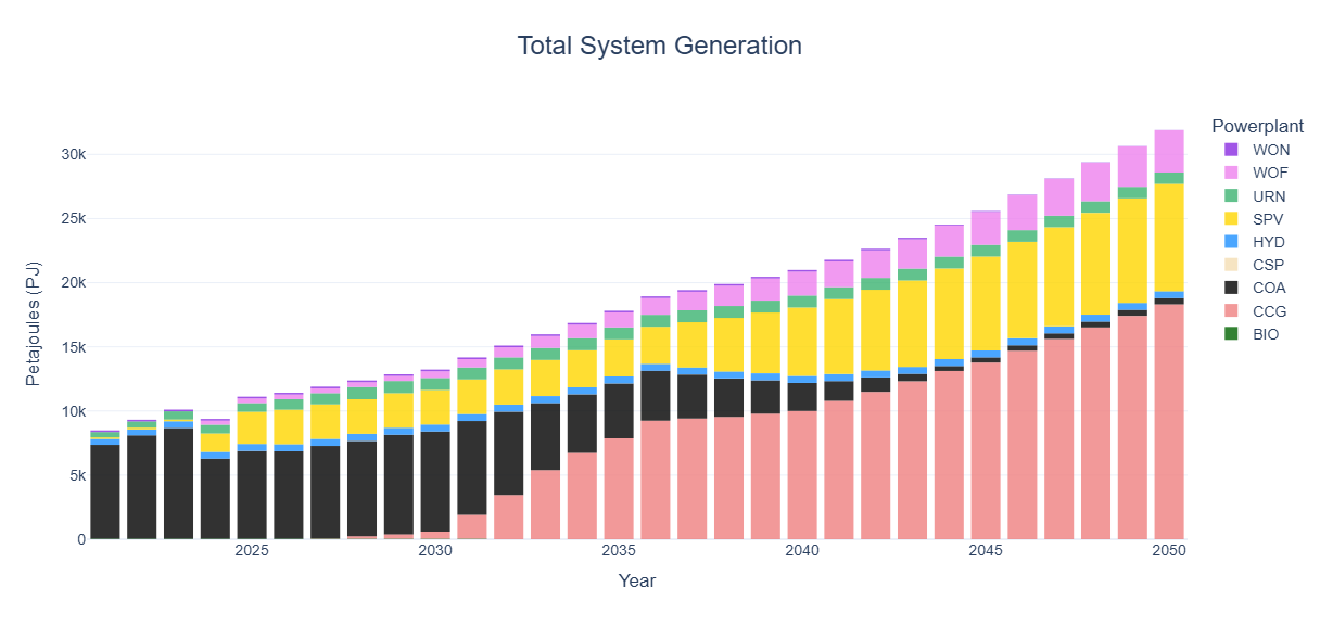
Navigate to the newly created results/ folder. All available automatically generated results are summarized below.

osemosys_global         
└── results        # Will appear after running the workflow
├── data       # Global CSV OSeMOSYS data     
├── figs       
│   ├── ...    # Global demand projections
└── India      # Name of scenario
    ├── data      # Scenario input CSV data
    ├── figures      # Result figures       
    │   ├── GenerationAnnual.html
    │   ├── GenerationHourly.html
    │   ├── TotalCapacityAnnual.html
    │   ├── TransmissionCapacity2050.jpg
    │   └── TransmissionFlow2050.jpg
    ├── result_summaries   # Auto generated result tables
    │   ├── AnnualEmissionIntensity.csv
    │   ├── AnnualEmissionIntensityGlobal.csv
    │   ├── AnnualExportTradeFlowsCountry.csv
    │   ├── AnnualExportTradeFlowsNode.csv
    │   ├── AnnualImportTradeFlowsCountry.csv
    │   ├── AnnualImportTradeFlowsNode.csv
    │   ├── AnnualNetTradeFlowsCountry.csv
    │   ├── AnnualNetTradeFlowsNode.csv
    │   ├── AnnualTotalTradeFlowsCountry.csv
    │   ├── AnnualTotalTradeFlowsNode.csv
    │   ├── GenerationSharesCountry.csv
    │   ├── GenerationSharesGlobal.csv
    │   ├── GenerationSharesNode.csv
    │   ├── Metrics.csv
    │   ├── PowerCapacityCountry.csv
    │   ├── PowerCapacityNode.csv
    │   ├── PowerCostCountry.csv
    │   ├── PowerCostGlobal.csv
    │   ├── PowerCostNode.csv
    │   ├── TotalCostCountry.csv
    │   ├── TotalCostGlobal.csv
    │   ├── TotalCostNode.csv
    │   ├── TradeFlowsCountry.csv
    │   ├── TradeFlowsNode.csv
    │   ├── TransmissionCapacityCountry.csv
    │   └── TransmissionCapacityNode.csv
    ├── results   # Scenario result CSV data
    └── India.txt  # Scenario OSeMOSYS data file              

File - figures	Description
`GenerationAnnual.html`	Plot of system level annual generation by technology
`GenerationHourly.html`	Plot of system level technology generation by timeslice
`TotalCapacityAnnual.html`	Plot of system level annual capacity by technology
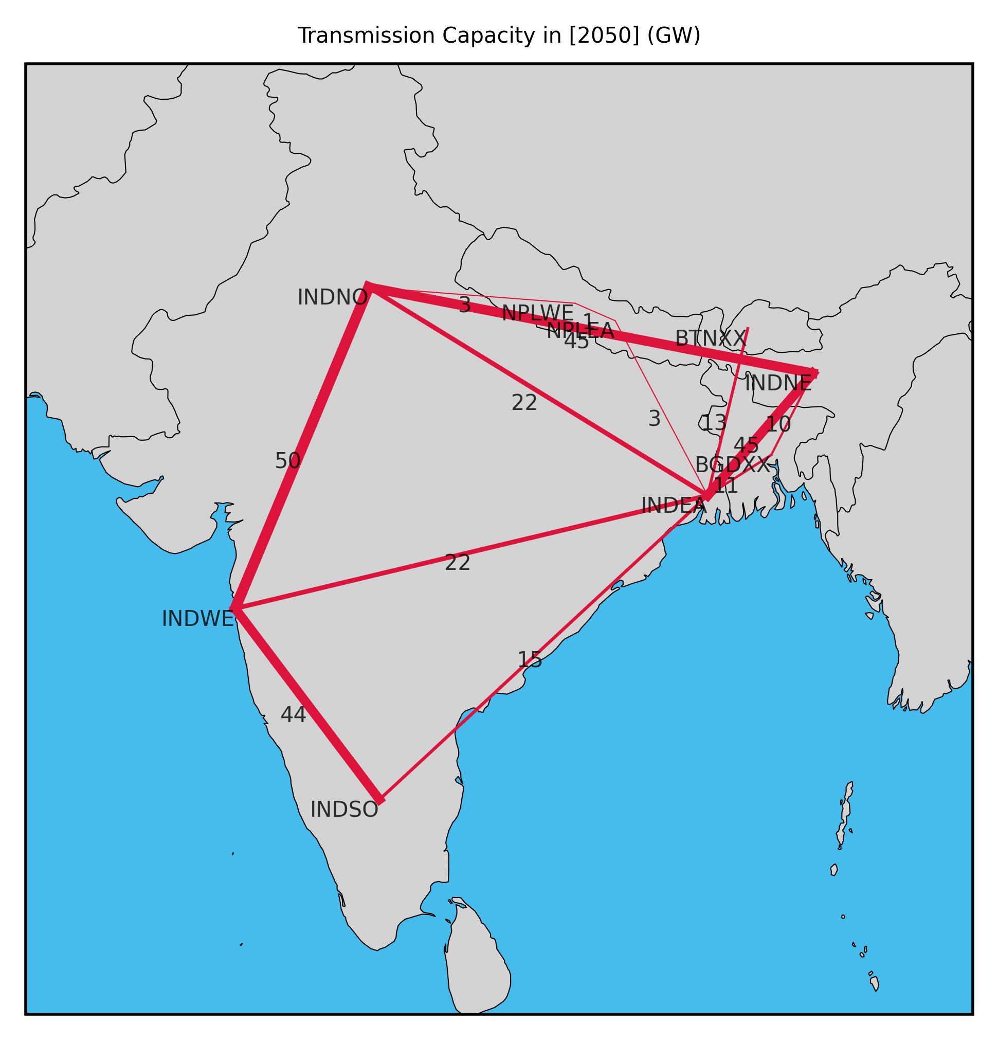
`TransmissionCapacityXXXX.jpg`	Transmission capacity plot for last year of model
`TransmissionFlowXXXX.jpg`	Transmission flow plot for last year of model

File - result_summaries	Description
`AnnualEmissionIntensity.csv`	Country level annual emission intensity (gCO2/kWh)
`AnnualEmissionIntensityGlobal.csv`	System level annual emission intensity (gCO2/kWh)
`AnnualExportTradeFlowsCountry.csv`	Country level annual electricity exports from node_1 to node_2 (PJ)
`AnnualExportTradeFlowsNode.csv`	Nodal level annual electricity exports from node_1 to node_2 (PJ)
`AnnualImportTradeFlowsCountry.csv`	Country level annual electricity exports from node_2 to node_1 (PJ)
`AnnualImportTradeFlowsNode.csv`	Nodal level annual electricity exports from node_2 to node_1 (PJ)
`AnnualNetTradeFlowsCountry.csv`	Country level annual net trade from node_1 to node_2 (PJ)
`AnnualNetTradeFlowsNode.csv`	Nodal level annual net trade from node_1 to node_2 (PJ)
`AnnualTotalTradeFlowsCountry.csv`	Country level annual total trade between node_1 and node_2 (PJ)
`AnnualTotalTradeFlowsNode.csv`	Nodal level annual total trade between node_1 and node_2 (PJ)
`GenerationSharesCountry.csv`	Country level annual generation shares per generator category (%)
`GenerationSharesGlobal.csv`	System level annual generation shares per generator category (%)
`GenerationSharesNode.csv`	Nodal level annual generation shares per generator category (%)
`Metrics.csv`	Summary statistics for the full model horizon
`PowerCapacityCountry.csv`	Country level annual capacity by technology (GW)
`PowerCapacityNode.csv`	Nodal level annual capacity by technology (GW)
`PowerCostCountry.csv`	Country level annual relative system cost ($/MWh, Total Costs / Demand)
`PowerCostGlobal.csv`	System level annual relative system cost ($/MWh, Total Costs / Demand)
`PowerCostNode.csv`	Nodal level annual relative system cost ($/MWh, Total Costs / Demand)
`TotalCostCountry.csv`	Country level total system cost ($M)
`TotalCostGlobal.csv`	System level total system cost ($M)
`TotalCostNode.csv`	Nodal level total system cost ($M)
`TradeFlowsCountry.csv`	Country level electricity trade by timeslice (PJ)
`TradeFlowsNode.csv`	Nodal level electricity trade by timeslice (PJ)
`TransmissionCapacityCountry.csv`	Country level annual transmission capacity (GW)
`TransmissionCapacityNode.csv`	Nodal level annual transmission capacity (GW)

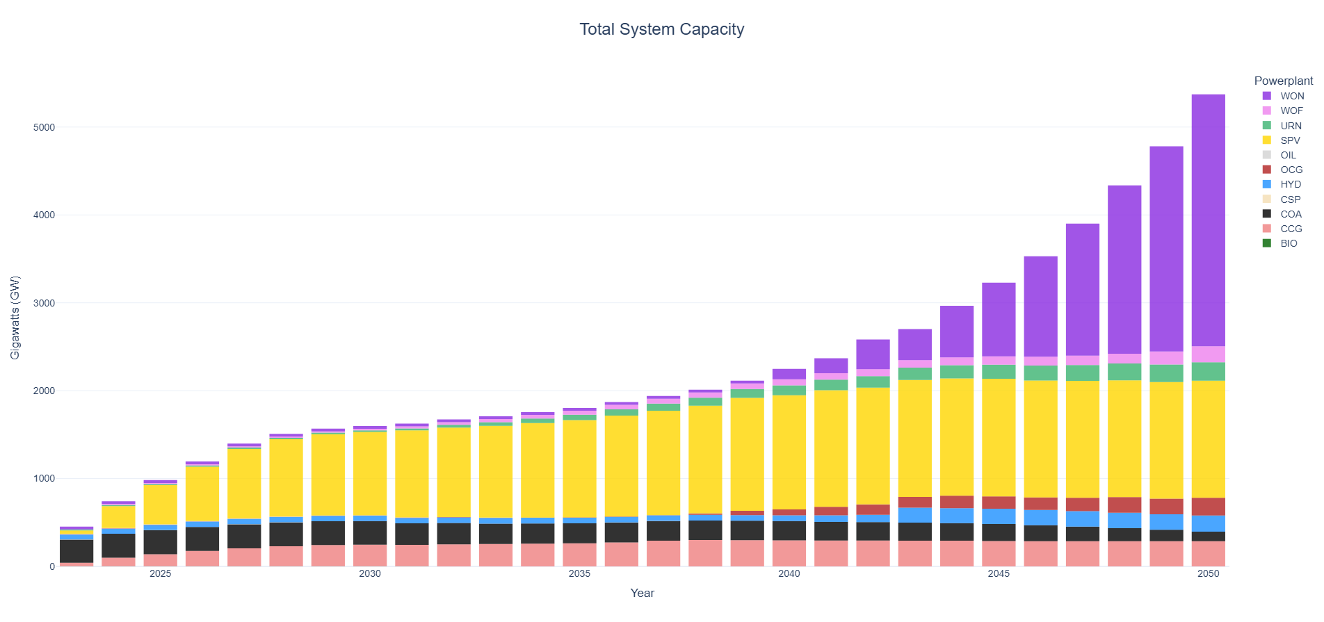
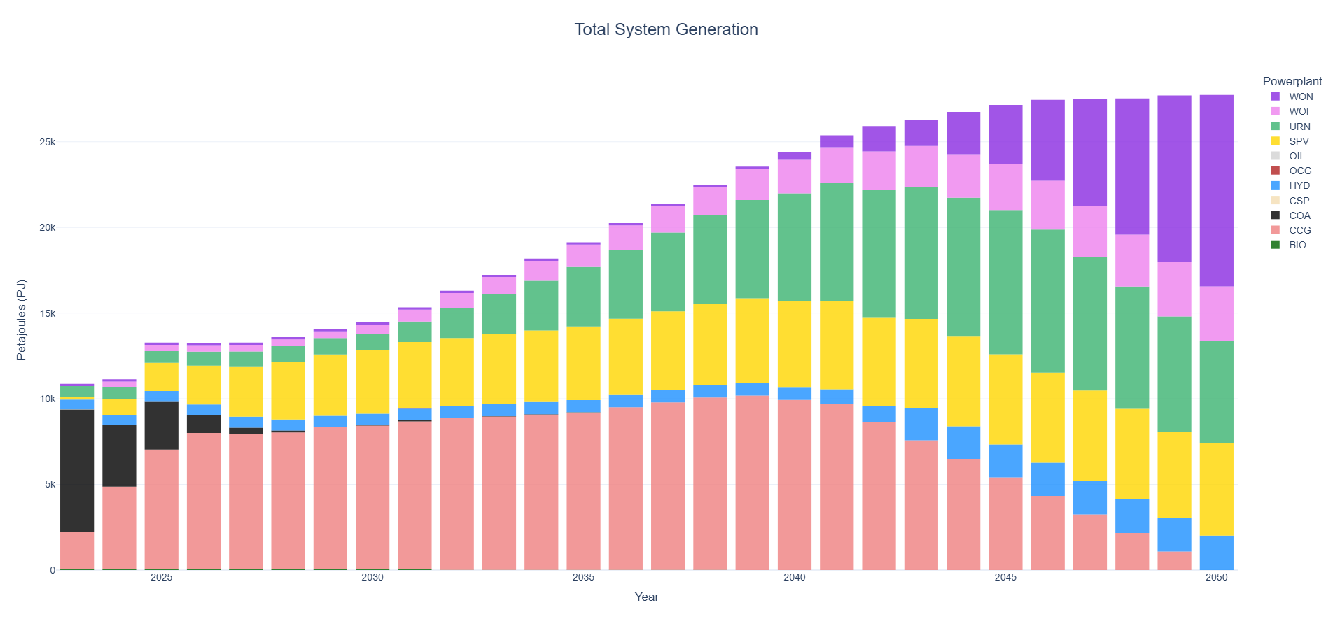
View system level capacity and generation results.

Caution

These results are used to showcase the capabilities of OSeMOSYS Global. The actual energy supply mix results will need further analysis, such as removing technology bias though implementing resource limits on solar-PV (SPV) and CCG (Combined Cycle Gas).

Tip

These plots are interactive! Hover over the bars to view values, or double click on a power plant in the legend to single it out.
View demand projections results in the file results/figs/projection.png. Grey dots represent historical country level values for countries in Asia and the coloured dots show projected values.

Example 2#

Goal: Modify the model geographic scope, temporal settings, emission penalty and generator build rates for CCG and SPV in India.

The goal of this scenario will be to change the geographic scope to add Bangladesh, Bhutan, and Nepal to the model. Moreover, we will change the model horizon to be from 2023-2050 and increase the number of time slices and seasons per year. We also set build rates for CCG at 10 GW/yr and to 5%/yr of the total solar PV potential in India. Finally, we will ensure cross border trade is allowed, set the emission penalty to $50/T, and create country level result plots.

Navigate to and open the file config/config.yaml
Change the scenario name to BBIN (Bangladesh, Bhutan, India, and Nepal)
```
scenario: 'BBIN'
```

Change the geographic scope to include the mentioned countries.

geographic_scope:
  - 'IND'
  - 'BGD'
  - 'BTN'
  - 'NPL'

Change the model horizon to be from 2023 to 2050. Both numbers are inclusive.
```
startYear: 2023
endYear: 2050
```
Change the number of day parts to represent three even 8 hour segments per day. The start number is inclusive, while the end number is exclusive.
```
dayparts:
  D1: [1, 9]
  D2: [9, 17]
  D3: [17, 25]
```
Change the number of seasons to represent 3 equally spaced days. All numbers are inclusive.
```
seasons:
  S1: [1, 2, 3, 4]
  S2: [5, 6, 7, 8]
  S3: [9, 10, 11, 12]
```
Tip

A timeslice structure of 3 seasons and 3 dayparts will result in a model with 9 timeslices per year; 3 representative days each with 3 timeslices.

See the OSeMOSYS documentation has more information on the OSeMOSYS timeslice parameters.
Ensure the crossborderTrade parameter is set to True
```
crossborderTrade: True
```

Change the emission penalty to 50 $/T and change the START_YEAR parameter to 2023.

emission_penalty:
  - ["CO2", "IND", 2023, 2050, 50]
  - ["CO2", "BGD", 2023, 2050, 50]
  - ["CO2", "BTN", 2023, 2050, 50]
  - ["CO2", "NPL", 2023, 2050, 50]

Adjust the generation build rates for CCG and SPV for India in data/custom/powerplant_build_rates.csv in GW.

TYPE

COUNTRY

METHOD

MAX_BUILD

START_YEAR

END_YEAR

CCG

IND

ABS

10

2024

2050

SPV

IND

PCT

5

2024

2050

Tip

Generator build rates can be set in absolute values (ABS) in GW or as a relative value (PCT) for renewables, where the % value set equals x % of the total resource potential for the specific technology and country. For the default OSeMOSYS Global nodes, resource potentials exist for HYD, SPV, WOF & WON. Custom resource potentials for all nodes (default and custom) and all renewables can be set in resources/data/custom/RE_potentials.csv.
Run the command snakemake -j6
```
(osemosys-global) ~/osemosys_global$ snakemake -j6
```
Tip

If you run into any issues with the workflow, run the command snakemake clean -c. This will delete any auto generated files and bring you back to a clean start.

TYPE	COUNTRY	METHOD	MAX_BUILD	START_YEAR	END_YEAR
CCG	IND	ABS	10	2024	2050
SPV	IND	PCT	5	2024	2050

Navigate to the results/ folder to view results from this model run.

Notice how under figures/, there is now a folder for each country. By setting the crossborderTrade parameter to be true, we tell the workflow to create out both system level and country level plots.

osemosys_global         
├── results        
│   ├── data       # Global CSV OSeMOSYS data     
│   ├── figs       
│   │   ├── ...    # Global demand projections
│   ├── BBIN      # Name of scenario
│   │   ├── data     # Scenario input CSV data
│   │   ├── figures      # Result figures
│   │   │   ├── BGD
│   │   │   │   ├── GenerationAnnual.html
│   │   │   │   ├── TotalCapacityAnnual.html     
│   │   │   ├── BTN
│   │   │   │   ├── GenerationAnnual.html
│   │   │   │   ├── TotalCapacityAnnual.html     
│   │   │   ├── IND
│   │   │   │   ├── GenerationAnnual.html
│   │   │   │   ├── TotalCapacityAnnual.html     
│   │   │   ├── NPL
│   │   │   │   ├── GenerationAnnual.html
│   │   │   │   ├── TotalCapacityAnnual.html     
│   │   │   ├── GenerationAnnual.html
│   │   │   ├── GenerationHourly.html
│   │   │   ├── TotalCapacityAnnual.html
│   │   │   ├── TransmissionCapacity2050.jpg
│   │   │   ├── TransmissionFlow2050.jpg
│   │   ├── result_summaries   # Auto generated result tables
│   │   ├── results   # Scenario result CSV data
│   │   ├── BBIN.txt  # Scenario OSeMOSYS data file               
└── ...

Note

If you don’t clean the model results, the previous scenario results are saved as long as you change the scenario name.

View system level 2050 hourly generation results by viewing the file results/BBIN/figures/GenerationHourly.html

Warning

When running the example model the below message is reported once the workflow is completed. Use of the BCK technology indicates that there is a supply shortage for the respective node (BGD).

The following Backstop Technologies are being used:

[‘PWRBCKBGDXX’]

Tip

By default time-series data in the OSeMOSYS Global workflow is reported in UTC+0. If you want to report values in a time-zone that is more applicable to the geographical scope for which the model is build you can use the timeshift parameter in the configuration file.

Example 3#

Goal: Validate the BBIN example and improve its accuracy based on historical data and adjust the model time-zone.

The goal of this scenario will be to rerun the BBIN scenario (example 2), except we will adjust some of its input parameters by comparing model outputs to historical data from benchmark datasets. We will furthermore adjust the time-zone to represent the local system.

Change the scenario name
```
scenario: 'BBINvalidated'
```
Change the timeshift paramater to UTC+6
```
timeshift: 6
```
View the capacity validation chart for BGD for 2023 located in
results/BBIN/validation/BGD/capacity/ember.png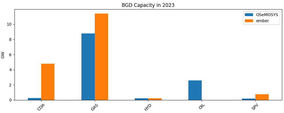

We can see that there is a significant capacity shortage for COA (± 4.5 GW), GAS (± 3 GW) and SPV (± 0.5 GW) in the OSeMOSYS Global outputs compared to the benchmark dataset (EMBER yearly electricity data).

Warning

The default data for generator capacity in OSeMOSYS Global for more recent years is currently not up to date. Validating and adjusting input data is recommended. Updating the OSeMOSYS Global workflow to more recent datasets is work in progress.
Adjust the existing capacities for COA, CCG and SPV for Bangladesh in resources/data/custom/residual_capacity.csv in MW. We will set values equal to the reported values in the benchmark dataset Ember yearly electricity data in MW values.

CUSTOM_NODE

FUEL_TYPE

START_YEAR

END_YEAR

CAPACITY

BGDXX

COA

2000

2030

4770

BGDXX

CCG

2000

2030

11390

BGDXX

SPV

2010

2040

770

CUSTOM_NODE	FUEL_TYPE	START_YEAR	END_YEAR	CAPACITY
BGDXX	COA	2000	2030	4770
BGDXX	CCG	2000	2030	11390
BGDXX	SPV	2010	2040	770

Run the command snakemake -j6

(osemosys-global) ~/osemosys_global$ snakemake -j6

Have another look at the validation chart for BGD for 2023 located in
results/BBINvalidated/validation/BGD/capacity/ember.png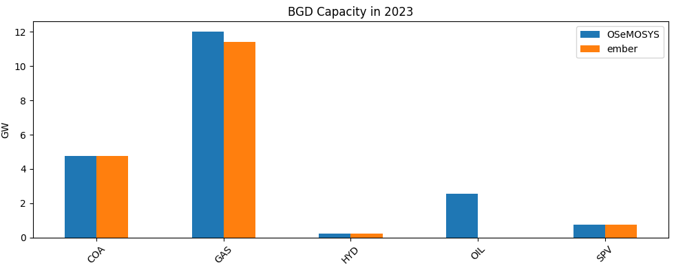

Warning

Eventhough the capacities are updated, we still see the use of the BCK technology in Bangladesh.

The following Backstop Technologies are being used:

[‘PWRBCKBGDXX’]

Tip

Further input changes can be made to adjust the total available supply. For example, by changing technology availability factors in
resources/data/custom/availability_factors.csv or by changing capacity factors for SPV in resources/data/custom/RE_profiles_SPV.csv. However, since there are limited renewables in Bangladesh in 2023 (the year of the supply shortage) and other technologies are used at a maximum rate it is an indicator that the projected electricity demand is overestimated.
Adjust the electricity demand for Bangladesh in 2023 in resources/data/custom/specified_annual_demand.csv. We will set values equal to the reported values in the benchmark dataset Ember yearly electricity data converted to PJ values.

CUSTOM_NODE

YEAR

VALUE

BGDXX

2023

416.052

CUSTOM_NODE	YEAR	VALUE
BGDXX	2023	416.052

Run the command snakemake -j6

(osemosys-global) ~/osemosys_global$ snakemake -j6

View system level 2050 hourly generation results by viewing the file results/BBINvalidated/figures/GenerationHourly.html to see the impact of the time-zone change.

View system level metrics for this model run by looking at the file results/BBINvalidated/result_summaries/Metrics.csv

Metric	Unit	Value
Emissions	Million tonnes of CO2-eq.	19946
Total System Cost	Billion $	1885
Cost of electricity	$/MWh	17
Fossil fuel share	%	46
Renewable energy share	%	50
Clean energy share	%	54

Example 4#

Goal: To add emission and renewable penetration targets that mimic potential pathways to a net-zero electricity system to the BBINvalidated scenario.

The goal of this scenario will be to add a range of different targets being 1) net-zero emission electricity targets for all BBIN countries, 2) a renewable generation target for Bangladesh and a WON capacity target for Southern India.

Caution

Emission, generation and capacity targets in OSeMOSYS Global are ‘hard’ constraints which means that once implemented they must be met. If this conflicts with other constraints in the model (e.g. generator build rates), this will lead to an infeasibility and the workflow will fail.

Revert back to the BBINvalidated scenario and change the scenario name
```
scenario: 'BBINtargets'
```
Add net-zero emission electricity targets for all countries by means of the emission_limit parameter.
```
emission_limit:
 - ["CO2", "IND", "LINEAR", 2050, 0]
 - ["CO2", "BGD", "LINEAR", 2050, 0]
 - ["CO2", "BTN", "LINEAR", 2050, 0]
 - ["CO2", "NPL", "LINEAR", 2050, 0]                 
```
Tip

Multiple emission limits can be set per country (single limit per year). If the emission_limit TYPE is set to LINEAR it means that an interpolated emission limit will be set for every year inbetween two limits (or the set limit and a historical value). If TYPE is set to POINT only the defined limit will be used with no emission limits in other years.
Add a 30 % renewable generation target (% of generation) from 2030 onwards for the combined output of 'SPV', 'WOF', 'WON' in Bangladesh.
```
re_targets:
  T01: ["BGD", ['SPV', 'WOF', 'WON'], "PCT", 2030, 2050, 30]           
```
Add a 100 GW capacity target by 2040 for Southern India for WON.
```
re_targets:
  T02: ["INDSO", ['WON'], "ABS", 2040, 2040, 100]           
```
Note

The last two letters in the region (ie. NO, NE, and EA for India, or XX for Nepal, Bhutan and Bangladesh) represent the node in each region. See our model structure document for more information on this.
Add a system reserve margin of 15 %. This is relevant to ensure security of supply in a system with high shares of variable renewables.
```
reserve_margin:
  RM1: [15, 2030, 2050]
```
Tip

The reserve_margin_technologies parameter allows you to set specific rerserve margin contributions (% of total capacity) of given technologies. This can be done for generator and storage technologies. Reserve margins in OSeMOSYS Global are applied at the system level.
Allow URN (Nuclear) to be a technology for which aditional capacity can be built. Some countries (e.g. Bangladesh) have known plans for further nuclear build-out.
```
no_invest_technologies: 
  - "CSP"
  - "WAV"
  - "OTH"
  - "WAS"
  - "COG" 
  - "GEO"
  - "BIO"
  - "PET"
```
Tip

The no_invest_technologies parameter determines which technologies are not allowed to be invested in. Note that capacities for future years can still occur if they are defined as residual capacities (for example within resources/data/custom/residual_capacity.csv.)

Run the command snakemake -j6

(osemosys-global) ~/osemosys_global$ snakemake -j6

View system level capacity and generation results.

Tip

Have a look at results\BBINtargets\result_summaries\GenerationSharesCountry.csv to see that the 30% renewable generation target in Bangladesh is met and have a look at results\BBINtargets\results\TotalCapacityAnnual.csv to see that the 100 GW Onshore Wind in Southern India target is met.

Example 5#

Goal: Add electricity storage to the BBINtargets model.

The goal of this scenario will be to add a Short Duration Storage (SDS) battery technology and a Long Duration Storage (LDS) storage technology to the model. We will also add user defined capacities for storage.

Change the scenario name
```
scenario: 'BBINstorage8hourly'
```
Change the storage_parameters paramater to include SDS with an assumed CAPEX cost of 1938 million dollar per GW, fixed cost of 44.25 million dollar per GW per yr, variable cost of 0 $ per MWh, a roundtrip efficiency of 85 % and a storage duration of 4 hours.

Then include LDS with an assumed CAPEX cost of 3794 million dollar per GW, fixed cost of 20.2 million dollar per GW per yr, variable cost of 0.58 $ per MWh, a roundtrip efficiency of 80 % and a storage duration of 10 hours.
```
storage_parameters:
  SDS: [1938, 44.25, 0, 85, 4] 
  LDS: [3794, 20.2, 0.58, 80, 10]
```
Tip

The storage duration parameter sets the link between the ‘generator’ component of a storage technology and the ‘storage/reservoir’ component. In essence, by setting a duration of 10 hours, we assume that every GW of power rating equals 10 GWh of storage. In other words, it will take the storage technology 10 hours to fully charge or discharge.
Ensure the storage_existing and storage_planned parameters are set to True which tells the model to make use of storage data from the Global Energy Storage Database in terms of existing and planned storage capacities.
```
storage_existing: True
```
```
storage_planned: True
```
Warning

OSeMOSYS Global requires technology names to be abbreviated in 3 letter codes (e.g. SDS, LDS). To make sure that the technology names as used in the Global Energy Storage Database are correctly transferred over into the workflow we need to define a correct technology mapping. This can be done in the workflow\scripts\osemosys_global\storage\constants.py file.

Add reserve margin contributions of the SDS and LDS technologies.

reserve_margin_technologies:
  LDS : 70
  SDS : 70   

Run the command snakemake -j6

(osemosys-global) ~/osemosys_global$ snakemake -j6

View system level capacity results for the storage technologies only.

Tip

By clicking on technologies in the legend, you can select or unselect entries on the interactive charts.
Change the scenario name
```
scenario: 'BBINstorage4hourly'
```
Change the number of day parts to represent 6 even 4 hour segments per day. The start number is inclusive, while the end number is exclusive.
```
dayparts:
  D1: [1, 5]
  D2: [5, 9]
  D3: [9, 13]
  D4: [13, 17]
  D5: [17, 21]
  D6: [21, 25]
```
Tip

Grab a coffee, this make take a little longer to run… More detailed dayparts and seasons can significantly increase model complexity and corresponding simulation time. On a common laptop while utilizing CBC as the solver it should take just over 20 minutes to solve.
View the system level capacity results to assess the impact of temporal resolution changes on the integration of electricity storage.

Example 6#

Goal: Add user defined capacities to the BBINstorage8hourly scenario.

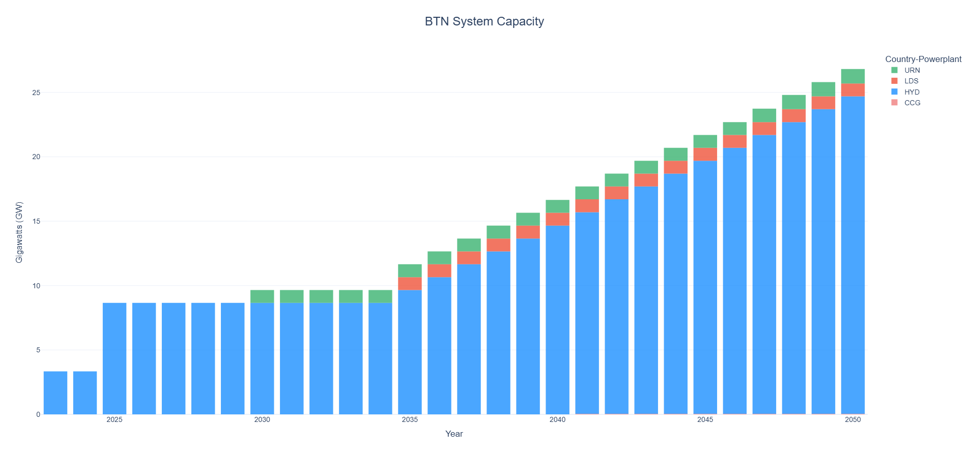
The goal of this scenario will be to add user defined capacities and parameters for power plants, storage and transmission. We will add a 1 GW Nuclear plant and a 3 GW Hydro plant to the system of Bhutan, a 3 GW transmission line between Bhutan and Eastern, India as well as a 1 GW LDS plant in Bhutan.

Change the scenario name
```
scenario: 'BBINuserdefined'
```
Change the number of day parts back to represent three even 8 hour segments per day. The start number is inclusive, while the end number is exclusive.
```
dayparts:
  D1: [1, 9]
  D2: [9, 17]
  D3: [17, 25]
```
Configure the new generators. We assume that the 3 GW HYD plant comes online in 2025 and that the 1 GW URN plant comes online in 2030. Furthermore, any new capacity afterwards can only be built starting in 2035 at max 1 GW per year with an associated CAPEX cost of 1000 million dollar per GW for HYD and 4400 for URN respectively. The assumed efficiency for the URN technology is 46 %.
```
user_defined_capacity:
  PWRHYDBTNXX01: [3, 2025, 2035, 1, 1000, 100]
  PWRURNBTNXX01: [1, 2030, 2035, 1, 4400, 46]
```
Caution

For any technology included in user_defined_capacity, the capacity and build_year parameters add residual capacity to the model for a given year. This is alongside residual capacities that are part of the default workflow or capacities that are entered in resources/data/custom/residual_capacity.csv. All other parameters overwrite the default values from the workflow (e.g. for efficiency) or substitute values defined elswhere (e.g. in resources/data/custom/powerplant_build_rates.csv).

Tip

For any renewable technology that includes seasonality (i.e. HYD, SPV, WON WOF) the efficiency parameter in user_defined_capacity is not binding (needs to be set between 0-100%). Custom monthly (HYD) or hourly (SPV, WON WOF) capacity factors for these technologies can be defined in resources/data/custom. For example for SPV this can be done in RE_profiles_SPV.csv.
Configure the new LDS plant. We assume that the 1 GW LDS plant comes online in 2035 with a further 1 GW per year allowed to be built in years after. Costs and efficiency parameters are kept equal to the default values for LDS as defined earlier in storage_parameters within (example 5).
```
user_defined_capacity_storage:
  sto1: [PWRLDSBTNXX01, 1, 2035, 2035, 1, 3794, 20.2, 0.58, 80]
```
Caution

Similar as to user_defined_capacity, the parameters within user_defined_capacity_storage related to residual capacities will add capacities to the workflow whereas the other parameters will overwrite values defined elsewhere (e.g. in resources/data/custom/storage_build_rates.csv or within storage_parameters).
Configure the new transmission line. We assume that the 3 GW line comes online in 2030. Furthermore, we assume that an additional 0.5 GW per year can be built between 2035 and 2050. Assumed CAPEX cost is 433 per GW, annual fixed O&M cost is 15.2 per GW per year, variable O&M cost (wheeling charge) is 4 $ per transmitted MWh and the assumed efficiency is 96.7 %.
```
user_defined_capacity_transmission:
  trn1: [TRNBTNXXINDEA, 3, 2030, 2035, 2050, 0.5, 433, 15.2, 4, 96.7]
```
Tip

The transmission_parameters parameter sets default values for common transmission technologies that can be adjusted by the user. For any potential transmission lines between default nodes, the OSeMOSYS Global workflow will automatically calculate costs and efficiency parameters that are distance and technology specific.

Caution

Do NOT delete the entries within transmission_parameters.

Caution

Similar as to user_defined_capacity and user_defined_capacity_storage, parameters related to residual capacities will add capacities to the workflow whereas the other parameters will overwrite values defined elsewhere (e.g. in resources/data/custom/transmission_build_rates.csv or within transmission_parameters).

Run the command snakemake -j6

(osemosys-global) ~/osemosys_global$ snakemake -j6

View the capacity results in Bhutan to see the effect of the user defined power plant and storage capacities.
View the transmission capacity plot in 2050 by looking at the file results/BBINuserdefined/figures/TransmissionCapacity2050.jpg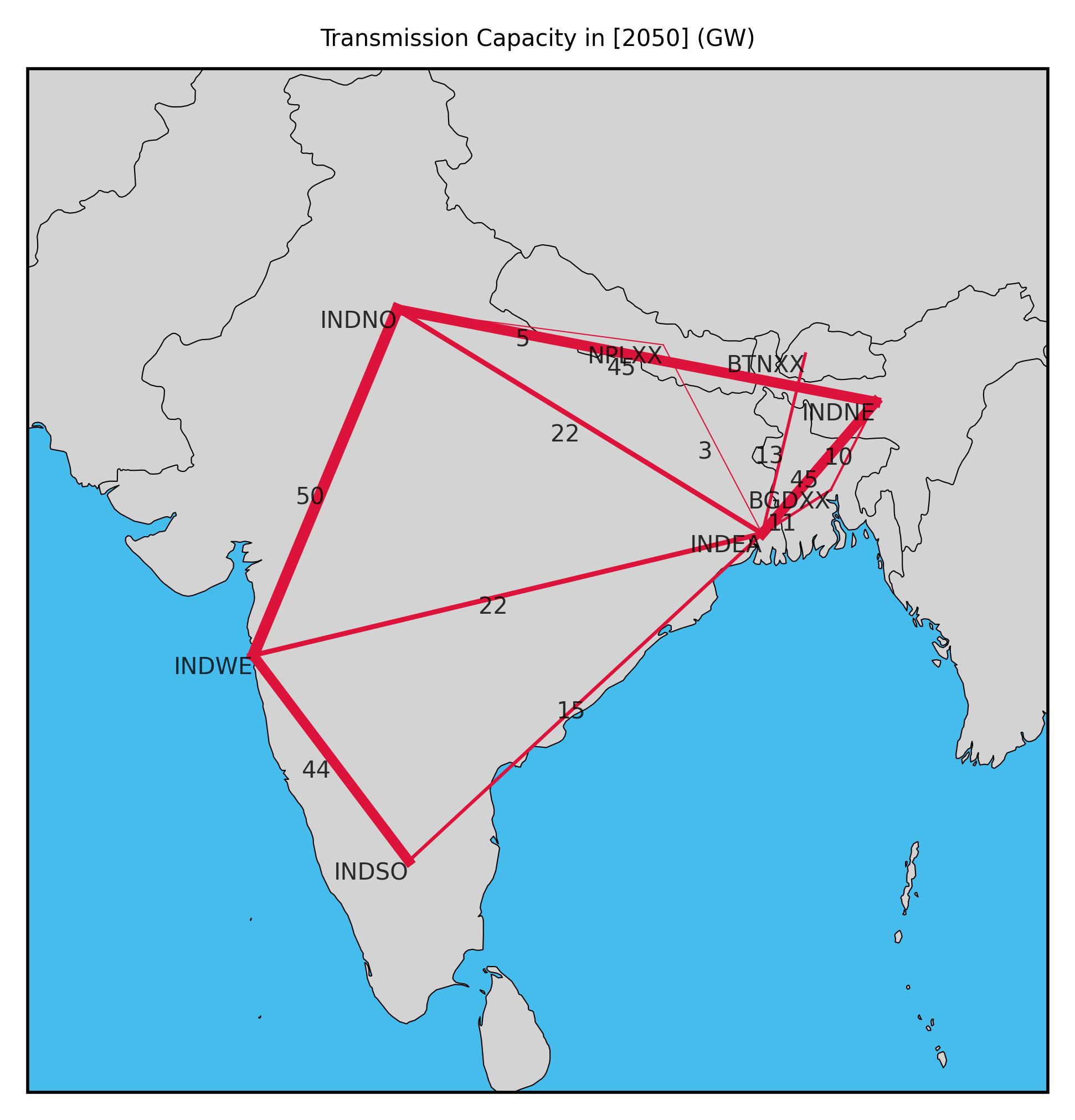
View the transmission flow plot in 2050 by looking at the file results/BBINuserdefined/figures/TransmissionFlow2050.jpg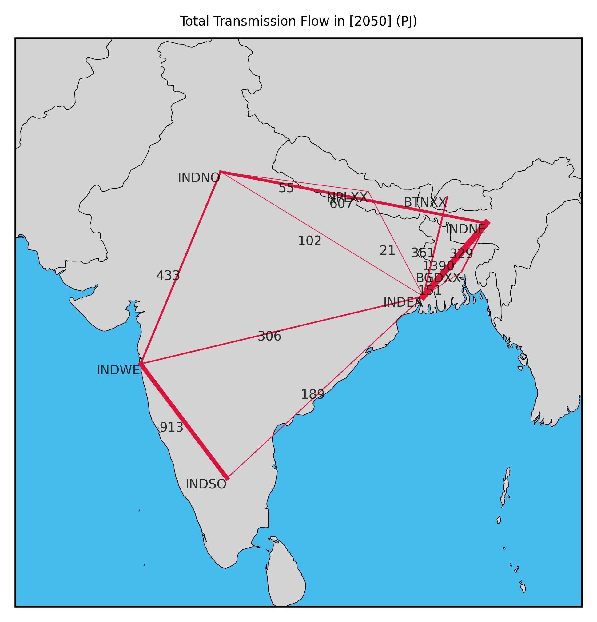

Example 7#

Goal: Add custom nodes to the model.

The goal of this scenario will be to alter the BBINuserdefined model by splitting Nepal into two seperate nodes being Eastern Nepal (NPLEA) and Western Nepal (NPLWE). We will add custom input data for the new model regions and will also add new transmission infrastruture between the new nodes as well as represent currently existing pathways between Nepal and other countries within BBIN.

Change the scenario name
```
scenario: 'BBINcustomregions'
```
Remove the country level node of Nepal from the model
```
nodes_to_remove:
 - "NPLXX"
```
Add the regional level nodes of Nepal to the model
```
nodes_to_add:
 - "NPLEA"
 - "NPLWE"
```
Warning

The custom nodes being added must start with the 3-letter code of the country that they are in (NPL in this case). Only the 2-letter regional code can change.

Caution

Do NOT delete NPL from the geographic_scope.
Add residual capacities in resources/data/custom/residual_capacity.csv. The fuel type must be one of the existing fuels in the model (see here) with capacities in MW. Do not remove other entries in the file.

CUSTOM_NODE

FUEL_TYPE

START_YEAR

END_YEAR

CAPACITY

NPLEA

HYD

2000

2080

1000

NPLWE

URN

2000

2060

1000

NPLWE

SPV

2025

2055

500
Add total resource potentials (GW) for renewables in resources/data/custom/RE_potentials.csv. Do not remove other entries in the file.

FUEL_TYPE

CUSTOM_NODE

CAPACITY

HYD

NPLEA

5

HYD

NPLWE

0

SPV

NPLEA

0

SPV

NPLWE

5

WON

NPLEA

0

WON

NPLWE

0

WOF

NPLEA

0

WOF

NPLWE

0

Note

For the purpose of this example, renewable potentials for other renewable technologies are set to 0 for exemplary purposes. When letting e.g. WON to be built without defining capacity factor timeseries for the custom nodes (see below) you essentially allow for a fully ‘dispatchable’ wind technology to be constructed as the model by default assumes 100% availabilty unless otherwise defined.
Add a monthly capacity factor timeseries for the HYD plant in NPLEA. For the purpose of this example, copy the profile from BTNXX and paste it into a new row. Set the NAME to NPLEA. Do not remove other entries in the file.

NAME

M1

M2

M3

M4

M5

M6

M7

M8

M9

M10

M11

M12

BTNXX

45.6

45.8

46.8

52.4

66.3

80

80

80

80

56.9

46.4

45.7

NPLEA

45.6

45.8

46.8

52.4

66.3

80

80

80

80

56.9

46.4

45.7
Add an hourly capacity factor timeseries for the SPV plant in NPLWE in resources/data/custom/RE_profiles_SPV.csv. For the purpose of this example, copy the profile from BTNXX and paste it into a new column. Set the column header to NPLWE. Do not remove other entries in the file.

Datetime

BTNXX

NPLWE

01/01/2015 0:00

0

0

01/01/2015 1:00

3.7

3.7

01/01/2015 2:00

12.7

12.7

01/01/2015 3:00

23.7

23.7

Note

Capacity factor profiles must be given for all hours in a single year. The data will then be aggregated according to the timeslice definition and replicated for each year.

Warning

The time-series for the example model are based on the 2015 climatic year. Profiles for different weather years can be used but the Datetime format needs to remain the same. Furthermore, the input timeseries need to be set in UTC+0 considering OSeMOSYS Global has a global scope. As shown in (example 3), the timeshift parameter can be used to shift the input profiles to a timezone that is more relevant for the geographic_scope of the model in question.
Add the annual electricity demand (PJ) for the new nodes in resources/data/custom_nodes/specified_annual_demand.csv. For the purpose of this example, copy the rows from BTNXX for ALL years and paste it into a new set of rows. Rename the CUSTOM_NODE entries to NPLEA. Repeat the same exercise but now for NPLWE. Do not remove other entries in the file. The table below shows an example, however users are required to add values for ALL model years (2023-2050).

CUSTOM_NODE

YEAR

CAPACITY

BTNXX

2021

9.5

BTNXX

2022

11.03

BTNXX

2023

12.58

NPLEA

2021

9.5

NPLEA

2022

11.03

NPLEA

2023

12.58

NPLWE

2021

9.5

NPLWE

2022

11.03

NPLWE

2023

12.58
Add the hourly specified demand profiles for the new nodes in resources/data/custom_nodes/specified_demand_profile.csv. For the purpose of this example, copy the profile from BTNXX and paste it into a new column. Set the column header to NPLEA. Repeat the same exercise but now for NPLWE. Do not remove other entries in the file.

Month

Day

Hour

BTNXX

NPLEA

NPLWE

1

1

0

0.00012

0.00012

0.00012

1

1

1

0.00013

0.00013

0.00013

1

1

2

0.00013

0.00013

0.00013

Tip

For each year, the fractional demand profiles for each node must sum up to 1.
Add the center points of the new nodes in resources/data/custom_nodes/centerpoints.csv. For Eastern Nepal we choose Kathmandu to be the center point and for Western Nepal we select Pokhara.

CUSTOM_NODE	FUEL_TYPE	START_YEAR	END_YEAR	CAPACITY
NPLEA	HYD	2000	2080	1000
NPLWE	URN	2000	2060	1000
NPLWE	SPV	2025	2055	500

FUEL_TYPE	CUSTOM_NODE	CAPACITY
HYD	NPLEA	5
HYD	NPLWE	0
SPV	NPLEA	0
SPV	NPLWE	5
WON	NPLEA	0
WON	NPLWE	0
WOF	NPLEA	0
WOF	NPLWE	0

NAME	M1	M2	M3	M4	M5	M6	M7	M8	M9	M10	M11	M12
BTNXX	45.6	45.8	46.8	52.4	66.3	80	80	80	80	56.9	46.4	45.7
NPLEA	45.6	45.8	46.8	52.4	66.3	80	80	80	80	56.9	46.4	45.7

Datetime	BTNXX	NPLWE
01/01/2015 0:00	0	0
01/01/2015 1:00	3.7	3.7
01/01/2015 2:00	12.7	12.7
01/01/2015 3:00	23.7	23.7

CUSTOM_NODE	YEAR	CAPACITY
BTNXX	2021	9.5
BTNXX	2022	11.03
BTNXX	2023	12.58
NPLEA	2021	9.5
NPLEA	2022	11.03
NPLEA	2023	12.58
NPLWE	2021	9.5
NPLWE	2022	11.03
NPLWE	2023	12.58

Month	Day	Hour	BTNXX	NPLEA	NPLWE
1	1	0	0.00012	0.00012	0.00012
1	1	1	0.00013	0.00013	0.00013
1	1	2	0.00013	0.00013	0.00013

region	lat	long
‘NPLEA’	27.700769	85.30014
‘NPLWE’	28.2096	83.9856

Tip

Center points in OSeMOSYS Global are used to calculate potential transmission distances between nodes. The default center points assume that transmission lines run between the largest population centers but users can make different assumptions. For example by picking geographical center points.

Following data from the Global Transmission Database existing and planned transmission capacity exists between Nepal and different parts of India. For the purpose of this study, we assume that Northern India is connected to Western Nepal and that Eastern India is connected to Eastern Nepal. We furthermore assume that a transmission line exists between Eastern and Western Nepal. Add the transmission objects to the model with the below assumptions. Do not remove the earlier defined transmission object.
```
user_defined_capacity_transmission:
  trn1: [TRNBTNXXINDEA, 3, 2030, 2035, 2050, 0.5, 433, 15.2, 4, 96.7]
  trn2: [TRNINDEANPLEA, 1, 2020, 2035, 2050, 0.5, 453, 15.9, 4, 96.4]
  trn3: [TRNINDEANPLEA, 2, 2028, 2035, 2050, 0.5, 453, 15.9, 4, 96.4]
  trn4: [TRNINDNONPLWE, 3, 2020, 2030, 2050, 0.5, 455, 15.9, 4, 96.4]
  trn5: [TRNNPLEANPLWE, 1, 2020, 2030, 2050, 0.5, 205, 7.2, 4, 99]
```
Warning

Following OSeMOSYS Global transmission naming standards, the name of a new transmission technology should be entered as TRN plus the combination of the node names in alphabetical order. For example TRNINDEANPLEA.

Tip

Multiple entries can be added for the same transmission object to represent residual capacities at different years. Note, this does require sequential key names (e.g. trn2, trn3).
Run the command snakemake -j6

(osemosys-global) ~/osemosys_global$ snakemake -j6

View the transmission capacity plot in 2050 by looking at the file to confirm that the custom nodes and transmission lines haven been added. results/BBINcustomregions/figures/TransmissionCapacity2050.jpg

Examples

Contents

Examples#

Example 1#

Example 2#

Example 3#

Example 4#

Example 5#

Example 6#

Example 7#